Verlet Integration – How do Dynamic Simulations work? – A Guide to Mathematical Studies (Archive)

Dynamic simulations play a crucial role in understanding and predicting the behavior of physical systems across various scientific and engineering disciplines. Whether modeling the movement of planets, simulating molecular dynamics, or creating realistic animations in computer graphics, the ability to accurately simulate dynamics is essential. One of the most effective and widely used methods for these simulations is Verlet integration. Known for its simplicity, accuracy, and stability, Verlet integration has become a cornerstone in the toolkit of computational scientists and engineers.

What is Verlet Integration?

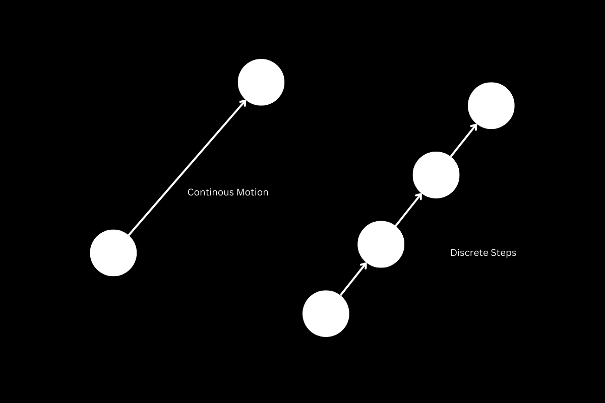
Verlet integration is a numerical method used to integrate Newton’s equations of motion. It is particularly well-suited for problems involving conservative forces, such as gravitational or electromagnetic forces, where energy conservation is important. The method calculates the positions of particles over time based on their initial positions, velocities, and the forces acting upon them. Unlike some other integration methods, Verlet integration uses both the current and previous positions of particles, avoiding direct computation of velocities and improving numerical stability.

The Mathematical Foundation

The basic form of Verlet integration can be derived from the Taylor expansion of the position of a particle. Let $\mathbf{r}(t)$ represent the position of a particle at time $t$ . The Taylor series expansions for the positions at $t + \Delta t$ and $t - \Delta t$ are:

$\mathbf{r}(t + \Delta t) = \mathbf{r}(t) + \mathbf{v}(t)\Delta t + \frac{1}{2}\mathbf{a}(t)(\Delta t)^2 + \mathcal{O}((\Delta t)^3)$

$\mathbf{r}(t - \Delta t) = \mathbf{r}(t) - \mathbf{v}(t)\Delta t + \frac{1}{2}\mathbf{a}(t)(\Delta t)^2 + \mathcal{O}((\Delta t)^3$

Adding these two equations cancels out the velocity term, resulting in:

$\mathbf{r}(t + \Delta t) = 2\mathbf{r}(t) - \mathbf{r}(t - \Delta t) + \mathbf{a}(t)(\Delta t)^2$

Here, $\mathbf{r}(t + \Delta t)$ is the position at the next time step, $\mathbf{r}(t)$ is the current position, $\mathbf{r}(t - \Delta t)$ is the position at the previous time step, and $\mathbf{a}(t)$ is the acceleration at the current time step. This approach leverages positions at two different times to compute the future position, providing a robust and accurate method for integrating the equations of motion.

Variants of Verlet Integration

Verlet integration has several variants, each tailored to specific needs:

Velocity Verlet: This variant includes explicit velocity calculations, which are useful for determining kinetic energy and other properties that depend on velocity. The positions and velocities are updated in a staggered manner to ensure consistency and stability. The updates follow these equations:

$\mathbf{r}(t + \Delta t) = \mathbf{r}(t) + \mathbf{v}(t)\Delta t + \frac{1}{2}\mathbf{a}(t)(\Delta t)^2$

$\mathbf{v}(t + \Delta t) = \mathbf{v}(t) + \frac{1}{2}[\mathbf{a}(t) + \mathbf{a}(t + \Delta t)]\Delta t$

Leapfrog Verlet: In this variant, velocities are updated at half-time steps, creating a leapfrog effect where positions and velocities are staggered in time:

$\mathbf{v}\left(t + \frac{\Delta t}{2}\right) = \mathbf{v}\left(t - \frac{\Delta t}{2}\right) + \mathbf{a}(t)\Delta t$

$\mathbf{r}(t + \Delta t) = \mathbf{r}(t) + \mathbf{v}\left(t + \frac{\Delta t}{2}\right)\Delta t$

This method enhances numerical stability and is particularly useful in molecular dynamics simulations.

Advantages of Verlet Integration

Verlet integration offers several advantages:

Stability: The method is known for its numerical stability, especially for small time steps. This is crucial when simulating physical systems over long durations, as it minimizes the accumulation of numerical errors.
Accuracy: By using positions at multiple time steps, Verlet integration reduces truncation errors, leading to more accurate results compared to simpler methods like Euler integration.
Simplicity: The algorithm is straightforward to implement and does not require explicit computation of velocities, simplifying the equations of motion and reducing computational overhead.

Applications of Verlet Integration

Verlet integration is employed in numerous fields due to its robustness and efficiency:

Molecular Dynamics: In molecular dynamics simulations, Verlet integration models interactions between atoms and molecules, helping scientists understand the structural and dynamical properties of materials, proteins, and other complex systems at the atomic level.
Computer Graphics: Verlet integration is crucial in physics engines for computer graphics, enabling realistic simulations of object movement, collisions, and other physical phenomena in virtual environments. It helps create lifelike animations in video games and movies.
Astrophysics: The method is used to simulate the motion of celestial bodies under gravitational forces. By integrating the equations of motion, scientists can predict the orbits of planets, moons, and other astronomical objects, aiding in the study of planetary systems and galaxy dynamics.
Biomechanics: In biomechanics, Verlet integration helps simulate the movement of biological systems, such as the human body, for studying gait, designing prosthetics, and understanding the mechanics of muscles and joints.
Robotics: In robotics, Verlet integration is used to simulate the dynamics of robots, helping engineers design and test control systems, predict robot behavior, and optimize performance.

Comparison with Other Integration Methods

While Verlet integration is widely favored for its stability and simplicity, it’s useful to compare it with other integration methods:

Euler Integration: The simplest method, updating positions using the current velocity and acceleration. While easy to implement, it suffers from significant numerical errors and stability issues, making it unsuitable for long-term simulations.
Runge-Kutta Methods: These methods offer higher accuracy by considering intermediate points within each time step. However, they are more computationally intensive and can be overkill for many physical simulations where Verlet integration provides sufficient accuracy.
Symplectic Integrators: Specifically designed for Hamiltonian systems, these integrators preserve the symplectic structure of the equations of motion, providing excellent long-term stability. Verlet integration is a simple form of symplectic integrator, which explains its stability in energy-conserving systems.

Implementation of Verlet Integration

Implementing Verlet integration involves iterating over time steps, updating positions, and accelerations as required. Below is a basic pseudocode for standard Verlet integration:

initialize positions r(t) and r(t - Δt)
initialize accelerations a(t)

for each time step Δt:
    compute new positions: r(t + Δt) = 2 * r(t) - r(t - Δt) + a(t) * (Δt)^2
    update previous position: r(t - Δt) = r(t)
    update current position: r(t) = r(t + Δt)
    compute new accelerations based on updated positions: a(t) = f(r(t)) / m

For Velocity Verlet:

initialize positions r(t) and velocities v(t)
initialize accelerations a(t)

for each time step Δt:
    compute new positions: r(t + Δt) = r(t) + v(t) * Δt + 0.5 * a(t) * (Δt)^2
    compute intermediate velocities: v(t + Δt/2) = v(t) + 0.5 * a(t) * Δt
    compute new accelerations based on updated positions: a(t + Δt) = f(r(t + Δt)) / m
    update velocities: v(t + Δt) = v(t + Δt/2) + 0.5 * a(t + Δt) * Δt

These implementations highlight the simplicity and efficiency of Verlet integration, making it a practical choice for dynamic simulations.

In conclusion, Verlet integration is a fundamental tool in the simulation of dynamic systems. Its ability to accurately and stably integrate equations of motion makes it indispensable in many scientific and engineering applications. From molecular dynamics to computer graphics and astrophysics, Verlet integration provides a reliable method for predicting the future states of physical systems. Understanding and implementing Verlet integration is essential for anyone involved in computational simulations of dynamic processes, offering a robust and efficient way to model the complexities of the physical world.

p.s. : This will be the end (for now) of the monthly series of mathematical articles. I am planning on repurposing this into a mathematics education site so stay tuned for more information!

Verlet Integration – How do Dynamic Simulations work?