An Introduction to Calculus – Limits and Differentiation – A Guide to Mathematical Studies (Archive)

Calculus – The type of mathematics that deals with rates of change, for example in the slope of a curve or the speed of a falling object.
Oxford Learner’s Dictionary

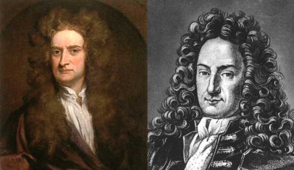
Although this definition would have been accurate at Newton or Leibniz’s time, there is no doubt it has since fallen short of the sheer scope of which modern-day calculus encompasses. From Fast-Fourier Transforms (FFTs) used in audio visualisations to Navier-Stokes equations modelling fluid dynamics, there is no aspect of mathematics which is more influential than calculus – it has defined modern mathematics and has established the basis of our technology. In this article, we will look at the basic building block of calculus – limits – and how they may be applied to solve real-life problems.

The official notation for a limit may be represented as follows : $lim_{x\rightarrow{n}} f(x)$ , where $n$ is the parameter of the function. In fact, we can define continuity of a certain region of a function this way if we can prove that the limit of the function at a certain arbitrary value is the actual value of the function at that point (in mathematical notation $lim_{n\rightarrow{x_0}} f(n)=f(x)$ , where $x_0$ is a value close to $x$ ).

The fundamental idea of limits stems from the fact that certain functions cannot be analytically calculated at certain points. For example if we wished to know what the behaviour of the function $f(x)=e^{-x}$ behaved at infinity, there is no way to directly calculate it – we cannot plug it into the equation and expect a numerical solution. However, if we plot the graph of $e^{-x}$ , we can clearly see that it is decaying towards $y=0$ . This can be proven using limits given that $f(x)$ is strictly decreasing – this can be proven easily using differentiation which we will discuss below:

$f(5)=6.74\cdot10^{-3}$
$f(20)=2.06\cdot10^{-9}$
$f(50)=1.93\cdot10^{-22}$
$f(100)=3.72\cdot10^{-44}$
∴ $lim_{x\rightarrow{\infty}}f(x)=0$

To better understand this, we may take $\lim_{x=0} \frac{sin(x)}{x}$ as an example – at $x=0$ the limit D.N.E. (does not exist) however if we look at the graph of $\frac{sin(x)}{x}$ we can see that actually the point does converge to a certain value, in this case 1. Readers who know l’Hopital’s rule may easily prove such a statement, however we are going to use the Squeeze Theorem to demonstrate a proof of the limit.

In this example, we may consider the area of △ABD ( $\frac{1}{2}\cdot{sin(x)}\cdot1$ ), sector ABD ( $\frac{x}{2\pi}\cdot\pi$ ) and △AFD ( $\frac{1}{2}\cdot{tan(x)}\cdot1$ ) simultaneously. From the diagram, we can clearly see that △ABD < sector ABD < △AFD, however by simplifying :

${\frac{1}{2}\cdot{sin(x)}\cdot1}\leq\frac{x}{2\pi}\cdot\pi\leq{\frac{1}{2}\cdot{tan(x)}\cdot1}$

$sin(x)\leq{x}\leq\frac{sin(x)}{cos(x)}$

$1\leq\frac{x}{sin(x)}\leq\frac{1}{cos(x)}$

$1\geq\frac{sin(x)}{x}\geq{cos(x)}$

As the upper limit of the inequality is 1 and the lower limit $\lim_{x=0}cos(x)=1$ , $\lim_{x=0} \frac{sin(x)}{x}$ must equal 1.

Now, to deem a function linearly continuous, the value of a certain point must be equal when approached from both sides – namely $\lim_{x=n^+}f(x)=\lim_{x=n^-}f(x)$ . These are named the left-hand and right-hand limit respectively, and is used to demonstrate that the function is continuous (at least over a certain interval).

Now, we can use this to estimate a slope of a function at a certain point. To start, let us take a look at a graph of a function, namely a quadratic of the form $\frac12{x^2+x-3}$ . The graph should look as such:

What could I do to find the slope of the equation at (2, 1)? First, we may recall the general equation of a slope between two points : $m=\frac{y_2-y_1}{x_2-x_1}$ , where $(x_1, y_1)$ and $(x_2, y_2)$ are points on a straight line. This can be manipulated to find the slope at a point of any equation. In the above scenario featuring the quadratic, we can find a random point on the function, for example (4, 9), and calculate the average gradient with the equation, namely $m_{(4, \text{ }9)}= \frac{9-1}{4-2}=4$ , shown by the blue line. However, we can use a closer point for a better estimation. Take the coordinates ( $3, \text{ }\frac92$ ) as another example. The coordinates would yield $m_{(3, \ \frac92)}=\frac{7}2$ as the green line, which as we can see from the graph is a better estimation than using the point (4, 9).

Using this logic, we can choose a much closer point to (2, 1) to obtain a very close approximation to the actual tangent. This can be generalised by the $x$ coordinate $x + {\Delta}x$ , where $\Delta{x}$ represents the change in the $x$ coordinate relative to the original coordinate, and the $y$ coordinates $f(x+\Delta{x})$ . This can be manipulated by limiting $\Delta{x}$ very close to 0, in mathematical notation $\lim_{\Delta{x}\rightarrow0}\Delta{x}$ . We can thus apply the slope equation, and obtain the following formula:

$\frac{d}{dx}f(x)=\lim_{\Delta{x}\rightarrow0}\frac{f(x+\Delta{x})-f(x)}{(x+\Delta{x})-{x}}=\lim_{\Delta{x}\rightarrow0}\frac{f(x+\Delta{x})-f(x)}{\Delta{x}}$

This formula is coined the first principles of differentiation, as it uses algebra as a basis for differentiation and allows for further development of calculus way beyond the scope of finding slopes. Now, we can utilise this formula to find the exact slope of the function at (2, 1) through substitution.

Example I : Find the equation of tangent at the point (2, 1) of the function $\frac12{x^2}+x-3$ .

By first principles:

$\frac{d}{dx}f(x)=\lim_{\Delta{x}\rightarrow0}\frac{[\frac12(x+\Delta{x})^2+(x+\Delta{x})-3]-[\frac12x^2+x-3]}{\Delta{x}}$

$=\lim_{\Delta{x}\rightarrow0}\frac{[\frac12x^2+\frac12(\Delta{x})^2+\frac12(2x\Delta{x})+x+\Delta{x}-3]-[\frac12x^2+x-3]}{\Delta{x}}$

$=\lim_{\Delta{x}\rightarrow0}\frac{\frac12x^2-\frac12x^2+x-x-3+3+x\Delta{x}+\Delta{x}+\frac12(\Delta{x})^2}{\Delta{x}}$

$=\lim_{{\Delta}x\rightarrow0}\frac{\frac12(\Delta{x})^2+x\Delta{x}+\Delta{x}}{\Delta{x}}=\lim_{{\Delta}x\rightarrow0}\frac12\Delta{x}+x+1$

$=\frac12{(\lim_{\Delta{x}\rightarrow0}\Delta{x}})+x+1=x+1$ ¹

Substituting $x=2$ as the $x$ coordinate, we get :

$\frac{d}{dx}f(2)=2+1=3$

This is the slope of the function at the point (2, 1).

Equation of the tangent :

$y-y_1=m(x-x_1)$

$y-1=3(x-2)$

$y-1=3x-6$

$y=3x-5$ Q.E.D.

As we can observe in the example, the operator $\frac{d}{dx}$ is used. This is the operator of differentiation in Leibniz notation. Multiple other notations are also used, such as $\frac{dy}{dx}$ , which symbolises $\frac{d}{dx}y$ , and also $f\prime(x)$ , which is read ‘f prime of $x$ ‘. These notations are used interchangeably, so it is much recommended to be familiar with them.

Using differentiation, we are also able to easily locate turning / stationary points of a function. These are the maximum or minimum points of a function. Take the function $\frac12{x^2}+x-3$ as an example. As we know the turning point must have slope 0, we can take the differentiation of the function and substitute $\frac{dy}{dx}=0$ .

$\frac{dy}{dx}=x+1$

$0=x+1$

$x=-1$

This indicates that the turning point of the function occurs at $x$ coordinate $-1$ . We can substitute this into the function and solve for $y$ .

$y=\frac12{(-1)^2}+(-1)-3$

$y=\frac12-1-3$

$y=-\frac{5}2$

Hence, we know that the turning point of the function is located at the coordinates ( $-1, \text{ }\frac52$ ).

We can also determine the nature of the turning point, i.e. whether it is a maximum or minimum point through taking the second derivative of the function, notated as $\frac{d^2y}{dx^2}$ . This can be generalised as follows:

If $\frac{d^2y}{dx^2}>0$ , it is a minimum point.
If $\frac{d^2y}{dx^2}<0$ , it is a maximum point.
If $\frac{d^2y}{dx^2}>0$ , the result is a saddle point – these are stable points where the function has a local maximum in one direction, but a local minimum in another direction (recall left-hand and right-hand limits).

Using all of this, we can now apply differentiation in real-life situations to solve different problems. Below are a few examples :

(Columbia University Calculus III Final 2013)

To solve this problem, we must first identify the relevant variables in the question, namely the radius $r$ and the height $h$ . We can then establish two equations:

Volume = $\pi{r}^2h=100\pi \longrightarrow{r^2}h=100\longrightarrow{h}=\frac{100}{r^2}$

Surface area = $\pi{r}^2+2\pi{r}h$

We can thus substitute the first equation into the second equation and obtain an equation for surface area entirely dependent of height.

Surface area = $\pi{r}^2+2\pi{r}(\frac{100}{r^2})$ = $\pi{r^2}+\frac{200\pi}{r}$

Now, in order to minimise surface area, we can take the differentiation of the equation with respect to radius and set $\frac{dA}{dr}=0$ (where $A$ symbolises area).

$\frac{dA}{dr}=2\pi{r}-200\pi{r}^{-2}$

$x0=2\pi{r}-200\pi{r}^{-2}$

$r^3=100 \longrightarrow{r}=\sqrt[3]{100}$ cm

We can then substitute the value back into the original equation to obtain the height.

${h}=\frac{100}{r^2}=\frac{100}{(\sqrt[3]{100})^2}=\sqrt[3]{100}$ cm

In conclusion, we’ve explored the fascinating world of limits and differentiations in calculus. We’ve delved into the fundamental concepts that underpin this branch of mathematics, from the intuitive idea of a limit to the precise techniques of differentiation. Hopefully, you’ve gained a deeper understanding of how calculus plays a pivotal role in analyzing change and motion.

But our journey through calculus is far from over. In our next installment, we’ll shift our focus to the counterpart of differentiation – integration. Just as differentiation helps us dissect complex functions and understand rates of change, integration enables us to piece together the pieces of information and find the cumulative effects over an interval.

So, stay tuned as we venture into the world of integration, where we’ll explore the concept of the integral, different techniques of integration, and its practical applications in various fields. Calculus is a powerful tool with immense relevance in science, engineering, economics, and beyond, and our exploration is just getting started.

Thank you for joining us on this mathematical journey, and I look forward to unraveling the mysteries of integration with you in our next article. Until then, keep exploring, keep learning, and keep pushing the boundaries of your mathematical knowledge!

It is important to note that $\lim_{x\rightarrow0}x=0$ . ↩︎

An Introduction to Calculus – Limits and Differentiation

Comments

Leave a Reply Cancel reply